Depending on what you are going to be using that data for, it’s very possible that you will need to sort data by only one string of information, and having it split into different cells makes that much easier to accomplish. But you can also run into situations where you need to combine your data, which you can accomplish with a very useful Excel formula called “Concatenate.” Our tutorial below will tell you more about this process.
How to Combine Three Columns in Excel 2013
Our article continues below with additional information and pictures of these steps. Need to combine some cells in Microsoft Word? Check out our tutorial on how to merge table cells in Word. Excel 2013 makes it possible for you to automatically generate and combine data that you have already entered into your spreadsheet. One way that you can do this is the CONCATENATE formula, which allows you to combine three columns into one in Excel. This is a powerful Excel tool to know, as it can help to eliminate a lot of wasted time. Once you have familiarized yourself with the formula and can use it to combine multiple cells into one, you can really expedite and eliminate a lot of tedious data entry that might have been taking up a lot of your time. Our guide below is going to walk you through setting up and customizing the CONCATENATE formula so that you can combine multiple columns into one in Excel. You may also be interested in our how to expand all columns in Excel tutorial if you find that you have information that is overlapping other cells.
How to Merge Three Columns Into One in Excel (Guide with Pictures)
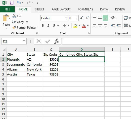
The steps below were performed in Excel 2013, but will also work for other versions of Excel. Note that we will show you how to do the basic formula that combines data from multiple cells, then we will show you how to modify it to include things like spaces and commas. This specific example will combine a city, state, and zip code into one cell. Now that you know how to combine three columns in Excel you will be able to fix a lot of issues that you might have previously needed to fix with a lot of retyping. At this point your data might just be one long string of text, which isn’t useful in certain situations. We can fix this by including some additional parts in the CONCATENATE formula. I am going to modify the formula for the data above so that I get a result that looks like Phoenix, AZ 85001 instead of PhoenixAZ85001. Note that there is a space after the comma in the first set of quotation marks, and a space between the second set of quotation marks. Our Microsoft Excel add column tutorial can show you ways to add values in multiple cells of a column very quickly.
Additional Notes
The cells do not have to be in this order. You could modify the formula to be =CONCATENATE(CC, AA, BB) or any other variation. Updating the data in one of the original, uncombined cells will cause that data to update automatically in the combined cell. If you need to copy and paste this combined data into another spreadsheet or a different worksheet, you might want to use the “Paste as text” option, otherwise the data might change if you adjust it after pasting. The method isn’t limited to just two or three columns. You can modify the formula as needed to include a very large amount of data or columns, depending on what you need to do.
Learn about using the VLOOKUP formula in Excel for some helpful ways to search for data and include it in cells more efficiently. You would click inside a cell in the target “combined column” where you wish to merge data. You can then type the array formula =CONCATENATE(AA, BB), but replace the placeholder single cell references with all the cells that you want to combine in the destination column. This will then display a string of data in the merged column that includes all of the content from those cells. For example, I could combine the first row of cells from column a to column e with the following formula – =CONCATENATE(A1, B1, C1, D1, E1) This is a pretty versatile formula and you can use it to show a lot of data from different cells in a single column. You would just need to modify the cell reference to include the worksheet name. For example, if I wanted to combine cell A1 in my current worksheet and cell A2 from a worksheet titled “Sheet2” then the formula would be: =CONCATENATE(A1, ‘Sheet2’!A2) After receiving his Bachelor’s and Master’s degrees in Computer Science he spent several years working in IT management for small businesses. However, he now works full time writing content online and creating websites. His main writing topics include iPhones, Microsoft Office, Google Apps, Android, and Photoshop, but he has also written about many other tech topics as well. Read his full bio here.


title: “How To Combine Three Columns Into One In Excel” ShowToc: true date: “2022-10-30” author: “Carol Mizrahi”
Depending on what you are going to be using that data for, it’s very possible that you will need to sort data by only one string of information, and having it split into different cells makes that much easier to accomplish. But you can also run into situations where you need to combine your data, which you can accomplish with a very useful Excel formula called “Concatenate.” Our tutorial below will tell you more about this process.
How to Combine Three Columns in Excel 2013
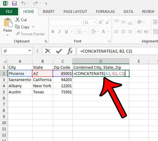
Our article continues below with additional information and pictures of these steps. Need to combine some cells in Microsoft Word? Check out our tutorial on how to merge table cells in Word. Excel 2013 makes it possible for you to automatically generate and combine data that you have already entered into your spreadsheet. One way that you can do this is the CONCATENATE formula, which allows you to combine three columns into one in Excel. This is a powerful Excel tool to know, as it can help to eliminate a lot of wasted time. Once you have familiarized yourself with the formula and can use it to combine multiple cells into one, you can really expedite and eliminate a lot of tedious data entry that might have been taking up a lot of your time. Our guide below is going to walk you through setting up and customizing the CONCATENATE formula so that you can combine multiple columns into one in Excel. You may also be interested in our how to expand all columns in Excel tutorial if you find that you have information that is overlapping other cells.
How to Merge Three Columns Into One in Excel (Guide with Pictures)
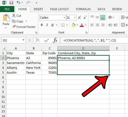
The steps below were performed in Excel 2013, but will also work for other versions of Excel. Note that we will show you how to do the basic formula that combines data from multiple cells, then we will show you how to modify it to include things like spaces and commas. This specific example will combine a city, state, and zip code into one cell. Now that you know how to combine three columns in Excel you will be able to fix a lot of issues that you might have previously needed to fix with a lot of retyping. At this point your data might just be one long string of text, which isn’t useful in certain situations. We can fix this by including some additional parts in the CONCATENATE formula. I am going to modify the formula for the data above so that I get a result that looks like Phoenix, AZ 85001 instead of PhoenixAZ85001. Note that there is a space after the comma in the first set of quotation marks, and a space between the second set of quotation marks. Our Microsoft Excel add column tutorial can show you ways to add values in multiple cells of a column very quickly.
Additional Notes
The cells do not have to be in this order. You could modify the formula to be =CONCATENATE(CC, AA, BB) or any other variation. Updating the data in one of the original, uncombined cells will cause that data to update automatically in the combined cell. If you need to copy and paste this combined data into another spreadsheet or a different worksheet, you might want to use the “Paste as text” option, otherwise the data might change if you adjust it after pasting. The method isn’t limited to just two or three columns. You can modify the formula as needed to include a very large amount of data or columns, depending on what you need to do.
Learn about using the VLOOKUP formula in Excel for some helpful ways to search for data and include it in cells more efficiently. You would click inside a cell in the target “combined column” where you wish to merge data. You can then type the array formula =CONCATENATE(AA, BB), but replace the placeholder single cell references with all the cells that you want to combine in the destination column. This will then display a string of data in the merged column that includes all of the content from those cells. For example, I could combine the first row of cells from column a to column e with the following formula – =CONCATENATE(A1, B1, C1, D1, E1) This is a pretty versatile formula and you can use it to show a lot of data from different cells in a single column. You would just need to modify the cell reference to include the worksheet name. For example, if I wanted to combine cell A1 in my current worksheet and cell A2 from a worksheet titled “Sheet2” then the formula would be: =CONCATENATE(A1, ‘Sheet2’!A2) After receiving his Bachelor’s and Master’s degrees in Computer Science he spent several years working in IT management for small businesses. However, he now works full time writing content online and creating websites. His main writing topics include iPhones, Microsoft Office, Google Apps, Android, and Photoshop, but he has also written about many other tech topics as well. Read his full bio here.
