There are times when you don’t want to show some data, but you also don’t want to get rid of it entirely. Our tutorial on how to hide cells in Excel continues below with more information on changing the appearance of your data.
How to Hide Columns in Excel 2013 (Or Rows)
Our guide continues below with more information on hiding cells in Excel 2013, including pictures of these steps. If you have worked with spreadsheets in Microsoft Excel or Google Sheets, then you may have encountered a worksheet where someone hid some of the data. Or maybe you even did it yourself, either intentionally or by accident, and wanted to know how or why it happened. Some spreadsheets that you edit in Microsoft Excel 2013 will contain an extraordinary amount of columns. For example, many of the spreadsheets that I create or modify in my day job come from online product databases, and it is not uncommon for these sheets to have dozens or hundreds of columns. But your current needs may not require all of that data, and you might need to remove some of it in order to show the data that is currently the most relevant. You may not want to delete that data, though, especially if it is part of a formula, or might be important later. One way to get your desired results is by hiding rows or columns that you don’t currently need. There are two different ways to hide rows or columns in Excel 2013, and we will show you both of those methods below.
How to Hide Rows in Excel 2013 (or Columns) – Guide with Pictures
The steps below are going to remove a row or column from view in your spreadsheet. This data is still actually there, so if you have a formula that is referencing a cell in one of the hidden rows or columns, that formula will not be affected. Additionally, if you copy a group of rows or columns and paste them into a new worksheet or a new workbook, those rows or columns will be copied as well and will be visible when you paste them.
Step 1: Open the spreadsheet containing the row or column that you wish to hide.
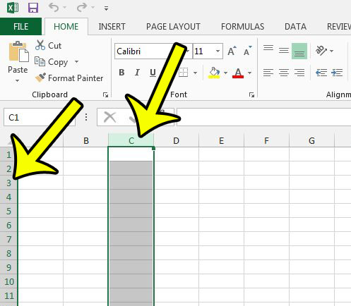
Step 2: Click the row number or the column letter of the row or column that you wish to hide.
If you don’t see row numbers or column letters, then read this article to see how you can unhide them.
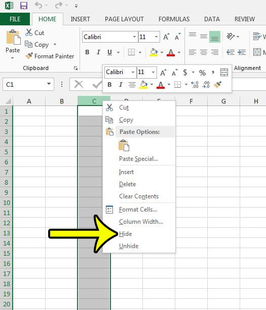
Step 3: Right-click the selected row number or column letter, or the selected rows or selected columns, then click the Hide option.
Note that you can use this same method if you need to hide multiple rows or columns. Simply click and hold on the first row number or column letter that you want to hide, then drag your mouse to select the rest of the rows or columns to hide. You can then right-click one of the selected rows or columns and choose the Hide option to hide all of them. Rows or columns can be hidden in a different manner as well, which we will discuss in the section below.
Alternate Method to Hide Rows or Columns in Excel 2013
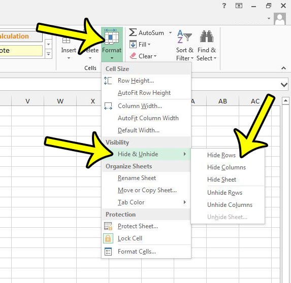
The steps described in this section will focus on using the Formats drop down menu on the Home tab to hide the row or column that you select.
Step 1: Select the row or column to hide.
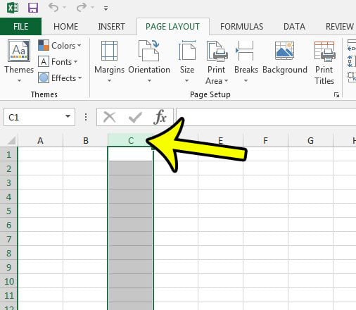
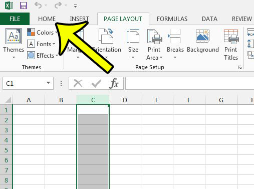
Step 2: Click the Home tab at the top of the window.
Step 3: Click the Format button in the Cells section of the ribbon, click Hide & Unhide, then click Hide Rows or Hide Columns, based on what is currently selected.
Why Would Anyone Want Hidden Rows or Hidden Columns in Microsoft Excel?
When your spreadsheet has a lot of rows and columns, then a hidden row or hidden column can be appealing for a couple of reasons. First, the ability to hide one or more columns or one or more rows is useful as a space-saving measure. It’s possible that your dataset includes a lot of information that you don’t need for your current activities, so being able to hide adjacent columns and focus on the data next to one row header or under one column header can be surprisingly useful. Second, there may be other people that are viewing or editing your Excel file. If you have a cell content with important data that shouldn’t be edited, then being able to hide cell contents will make it more difficult for people to edit or delete that data.
More Information on How to Hide Cells in Excel 2013
The steps in our tutorial above provide you with ways of hiding cells in an Excel spreadsheet. Unfortunately, you aren’t able to pick and choose specific cells that you want to hide. Instead, you are limited to hiding an entire row or an entire column. As we mentioned previously you can hide multiple rows or hide multiple columns using this same technique. To select multiple entities you can either hold down the Ctrl key on your keyboard and click each row number or column letter to hide, or you can click the first row or column to hide, hold down the Shift key, then click the last row or column to hide. If you need to unhide cells in Excel 2013 then you will need to click the row or column on one side of the hidden cells, hold down the Shift key, then click the row or column on the other side of the hidden cells. You can then right-click the selected range and choose the Unhide option. as with the alternate method we discussed above you can also unhide hidden cells by going to Home > Format > Hide & Unhide > then choose Unhide Rows or Unhide Columns. If there is a hidden row or a hidden column then there should be a small gap between the selected row headers or column headers. The numbering and lettering should also be skipping values. For example if you have a column header for A, B, and C, then it jumps to F, then columns D and E are hidden. Is there an entire worksheet, or worksheet tab, that you would like to hide from view in your Excel file? Read this article on hiding Excel worksheets so that you can remove an entire spreadsheet from view in your workbook.
He specializes in writing content about iPhones, Android devices, Microsoft Office, and many other popular applications and devices. Read his full bio here.
